
与其说深度学习是一门技术,不如说深度学习是一种语言
GitHub 项目地址:AI-Project/scratch
一、自动微分
1. 简单的例子
1.1 张量 x 的梯度
张量 $x$ 的梯度可以存储在 $x$ 上。
要点:
x.grad: 取$x$的梯度x.requires_grad_(True): 允许 tenser$x$存储自己的梯度x.grad.zero_(): 将$x$的梯度置零
import torch

# 初始化张量 x (tenser x)
x = torch.arange(4.0)

x.requires_grad_(True)  # 允许 tensor x 存储梯度
x.grad == None  # 梯度默认为 None
> True
初始化带梯度的张量,下面是两个例子:
torch.tensor([1., 2., 3.], requires_grad=True)
> tensor([1., 2., 3.], requires_grad=True)
torch.randn((2, 5), requires_grad=True)
> tensor([[ 0.4075, 1.1930, 0.5716, -1.0924, 0.0653], [-1.2869, 1.5768, 1.3445, 0.6309, -0.0484]], requires_grad=True)
1.2 损失函数 及 反向传播
我们约定:
- 将 损失 记为
$y$ - 设 损失函数 为:
$y = 2 * x \cdot x$(注意是点乘)
计算 $y$ 关于 $x$ 每个分量的梯度,步骤如下:
- 定义损失函数:
y = 2 * torch.dot(x, x) - 计算
$y$关于$x$的梯度,即反向传播:y.backward() - 获取更新后
$x$的梯度:x.grad
y = 2 * torch.dot(x, x)
y.backward()  # 用反向传播自动计算 y 关于 x 每个分量的梯度

x.grad
> tensor([ 0., 4., 8., 12.])
函数 $y = 2x^{T}x$ 关于 $x$ 的梯度应为 $4x$,验证是否正确:
x.grad == 4 * x
> tensor([True, True, True, True])
2. 当损失为向量时
梯度的“形状”:
- 当损失
$y$为 标量 时,梯度是 向量,且与$x$维度相同 - 当损失
$y$为 向量 时,梯度是 矩阵
注意,当损失 $y$ 为向量时。我们的目的不是计算微分矩阵,而是单独计算批量中每个样本的偏导数之和。也就是说:
在反向传播代码里要多加一个 sum() 函数,写成 y.sum().backward()
x.grad.zero_()  # 将张量 x 的梯度置零
x, x.grad
> (tensor([0., 1., 2., 3.], requires_grad=True), tensor([0., 0., 0., 0.]))
定义损失函数:$y = 2 * x \times x$(注意是叉乘)
# 定义损失函数
y = 2 * x * x
y  # 注意 y 在这里是向量
> tensor([ 0., 2., 8., 18.], grad_fn=<MulBackward0>)
y.sum().backward()
x.grad
> tensor([ 0., 4., 8., 12.])
3. with torch.no_grad()
在 PyTorch 中,如果一个张量的 requires_grad 参数设为 True。则所有依赖它的张量的 requires_grad 参数将被设置为 True
但在 with torch.no_grad() 块中的张量,依赖它的张量的 requires_grad 参数将被设为 False
参见:pytorch.org
下面是一个例子:
x = torch.tensor([1.], requires_grad=True)
with torch.no_grad():
    y = x * 2
y.requires_grad
> False
作为对照:
x = torch.tensor([1.], requires_grad=True)
y = x * 2
y.requires_grad
> True
二、加载数据
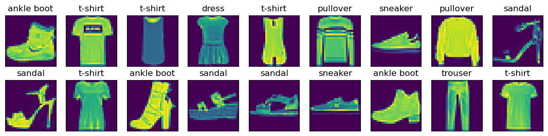
本节学习将 图像分类数据集 Fashion-MNIST 分割成训练集和测试集,并构造一个数据加载器 Generators 使得数据可以被多次迭代使用。
教程链接:image-classification-datasetv
%matplotlib inline
import time
import torch
import torchvision
from torch.utils import data
from torchvision import transforms
import matplotlib.pyplot as plt
1. 读取数据集
读取 Fashion-MNIST 数据集 (Xiao et al., 2017)
# 通过ToTensor实例将图像数据从PIL类型变换成32位浮点数格式,
# 并除以255使得所有像素的数值均在0~1之间
trans = transforms.ToTensor()
mnist_train = torchvision.datasets.FashionMNIST(
    root="../data", train=True, transform=trans, download=True)
mnist_test = torchvision.datasets.FashionMNIST(
    root="../data", train=False, transform=trans, download=True)
def get_fashion_mnist_labels(labels):  #@save
    """返回Fashion-MNIST数据集的文本标签"""
    text_labels = ['t-shirt', 'trouser', 'pullover', 'dress', 'coat',
                   'sandal', 'shirt', 'sneaker', 'bag', 'ankle boot']
    return [text_labels[int(i)] for i in labels]
def show_images(imgs, num_rows, num_cols, titles=None, scale=1.5):  #@save
    """绘制图像列表"""
    figsize = (num_cols * scale, num_rows * scale)
    _, axes = plt.subplots(num_rows, num_cols, figsize=figsize)
    axes = axes.flatten()
    for i, (ax, img) in enumerate(zip(axes, imgs)):
        if torch.is_tensor(img):
            # 图片张量
            ax.imshow(img.numpy())
        else:
            # PIL图片
            ax.imshow(img)
        ax.axes.get_xaxis().set_visible(False)
        ax.axes.get_yaxis().set_visible(False)
        if titles:
            ax.set_title(titles[i])
    return axes
X, y = next(iter(data.DataLoader(mnist_train, batch_size=18)))
X.shape, y.shape
> (torch.Size([18, 1, 28, 28]), torch.Size([18]))
show_images(X.reshape(18, 28, 28), 2, 9, titles=get_fashion_mnist_labels(y))
2. 读取小批量
在每次迭代中,数据加载器每次都会读取一小批量数据,大小为batch_size。 通过内置数据迭代器,我们可以随机打乱了所有样本,从而无偏见地读取小批量。
batch_size = 256

def get_dataloader_workers():  #@save
    """使用4个进程来读取数据"""
    return 4

train_iter = data.DataLoader(mnist_train, batch_size, shuffle=True,
                             num_workers=get_dataloader_workers())
class Timer:
    """Record multiple running times."""
    def __init__(self):
        """Defined in :numref:`sec_minibatch_sgd`"""
        self.times = []
        self.start()

    def start(self):
        """Start the timer."""
        self.tik = time.time()

    def stop(self):
        """Stop the timer and record the time in a list."""
        self.times.append(time.time() - self.tik)
        return self.times[-1]

    def avg(self):
        """Return the average time."""
        return sum(self.times) / len(self.times)

    def sum(self):
        """Return the sum of time."""
        return sum(self.times)

    def cumsum(self):
        """Return the accumulated time."""
        return np.array(self.times).cumsum().tolist()
# 看一下读取训练数据所需的时间
timer = Timer()
for X, y in train_iter:
    continue
f'{timer.stop():.2f} sec'
3. 整合所有组件
def load_data_fashion_mnist(batch_size, resize=None):
    """下载Fashion-MNIST数据集,然后将其加载到内存中"""
    trans = [transforms.ToTensor()]
    if resize:
        trans.insert(0, transforms.Resize(resize))
    trans = transforms.Compose(trans)
    mnist_train = torchvision.datasets.FashionMNIST(
        root="../data", train=True, transform=trans, download=True)
    mnist_test = torchvision.datasets.FashionMNIST(
        root="../data", train=False, transform=trans, download=True)
    return (data.DataLoader(mnist_train, batch_size, shuffle=True,
                            num_workers=get_dataloader_workers()),
            data.DataLoader(mnist_test, batch_size, shuffle=False,
                            num_workers=get_dataloader_workers()))
通过指定resize参数来测试load_data_fashion_mnist函数的图像大小调整功能
for X, y in train_iter:
    print(X.shape, X.dtype, y.shape, y.dtype)
    break
> torch.Size([256, 1, 28, 28]) torch.float32 torch.Size([256]) torch.int64
train_iter, test_iter = load_data_fashion_mnist(32, resize=64)
for X, y in train_iter:
    print(f"X.shape: {X.shape}")
    print(f"X.dtype: {X.dtype}")
    print(f"y.shape: {y.shape}")
    print(f"y.dtype: {y.dtype}")
    break
三、Logstic 回归
%matplotlib inline
import random
import math
import numpy as np
import collections
import matplotlib.pyplot as plt
from sklearn.linear_model import LogisticRegression
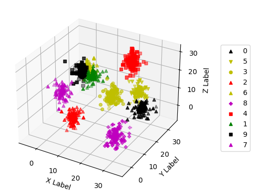
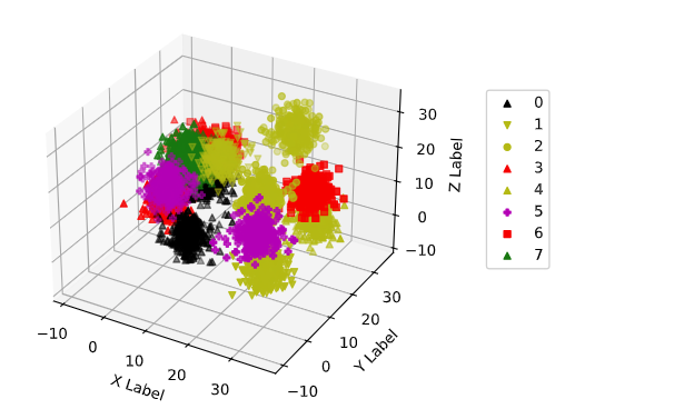
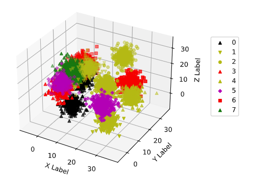
1. 生成样本和标号
# 画图参数
COLORS = ['b', 'g', 'r', 'c', 'm', 'y', 'k']
MARKERS = ['o', 'v', '^', 's', 'P']

# 业务参数
DIM = 3
CLUSTR_NUM = 10


def generate_sample(clustr_num, width=30, std=3, smin=600, smax=700, gen_seed=9603602):
    """生成样本
    clustr_num: 簇数
    width: 空间点位于长宽高均为 width 的正方体内
    std: 生成样本时,样本与样本中心距离的标准差
    smin: 生成样本量时,样本量的最小值
    smax: 生成样本量时,样本量的最大值
    """
    if clustr_num > len(COLORS) * len(MARKERS):
        raise Exception("Error: clustr_num <= len(COLORS) * len(MARKERS)")
    dim = DIM
    res = collections.defaultdict(list)

    random.seed(gen_seed)
    for i in range(clustr_num):
        mean = [random.random() * width for _ in range(dim)]
        sample_num = round((smax - smin) * random.random()) + smin
        for r in np.random.normal(0, std, sample_num):
            deg = [random.random() * math.pi * 2 for _ in range(2)]
            node = [mean[0] + r * math.cos(deg[0]) * math.cos(deg[1]),
                    mean[1] + r * math.cos(deg[0]) * math.sin(deg[1]),
                    mean[2] + r * math.sin(deg[0])]

            res[i].append(node)

    return res
samples = dict(generate_sample(clustr_num=CLUSTR_NUM))
# samples
def _3d_plot(samples):

    fig = plt.figure()
    ax = fig.add_subplot(projection='3d')

    mix = [(c, m) for c in COLORS for m in MARKERS]
    np.random.seed(19680801)
    np.random.shuffle(mix)
    for i, f in enumerate(samples.items()):
        k, v = f
        color, marker = mix[i]

        xs = [e[0] for e in v]
        ys = [e[1] for e in v]
        zs = [e[2] for e in v]
        ax.scatter(xs, ys, zs, color=color, marker=marker, label=k)

    ax.set_xlabel('X Label')
    ax.set_ylabel('Y Label')
    ax.set_zlabel('Z Label')
    ax.legend = ax.legend(bbox_to_anchor=(.5, .30, .85, .5))

    plt.show()
_3d_plot(samples)

2. 分割 训练集 和 预测集
def load_data(samples, div_rate=0.8):
    X, Y = [], []

    # 把输入整成适合sklearn输入的形状
    for lable, vlist in samples.items():
        for v in vlist:
            X.append(v)
            Y.append(lable)

    # 校验
    if not (div_rate <= 0.95 and div_rate > 0):
        raise Exception("Error: div_rate <= 0.95 and div_rate > 0")
    if len(X) != len(Y):
        raise Exception("Error: len(X) != len(Y)")

    # shuffle
    data = list(zip(X, Y))
    random.shuffle(data)
    X = [e[0] for e in data]
    Y = [e[1] for e in data]

    # 分割训练集和预测集
    div_num = math.floor(len(X) * div_rate)
    train_X, train_Y = X[:div_num], Y[:div_num]
    test_X, test_Y = X[div_num:], Y[div_num:]

    return train_X, train_Y, test_X, test_Y
train_X, train_Y, test_X, test_Y = load_data(samples)
sum(test_Y), len(test_Y)
> (5920, 1294)
train_X[:3], train_Y[:3], test_X[:3], test_Y[:3]
> ([[20.837554579645627, 18.961845823741736, 16.633726090847148], [2.3794870779388098, 28.838366976092825, 13.376753958471658], [4.851394029530915, 8.603495446318274, 17.186267813538862]], [3, 6, 7], [[29.404596908032293, 21.33132439225346, 6.65602456625498], [27.167331038537665, 27.64980912165818, 7.986085486917643], [19.193191406802836, 15.638041952359082, 7.5837088545045495]], [0, 5, 3])
3. 借助 sklearn 的简单实现
sklearn链接:sklearn.linear_model.LogisticRegression
logreg = LogisticRegression(C=1e5, max_iter=100000)
logreg.fit(train_X, train_Y)
pred_Y = logreg.predict(test_X)
pred_Y
> array([0, 5, 3, ..., 5, 2, 1])
def simple_accuracy(pred_Y, test_Y):
    l = [int(y==y_hat) for y, y_hat in zip(test_Y, pred_Y)]
    l_sum = sum(l)
    return l_sum, len(l), round(l_sum / len(l), 4)
pos, s, acc = simple_accuracy(pred_Y, test_Y)
print("预测正确的个数:", pos)
print("总数:", s)
print("精确率:", acc)
> 预测正确的个数: 1223 总数: 1294 精确率: 0.9451
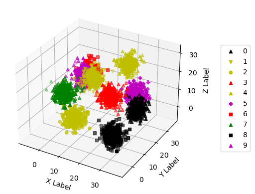
pred_samples = collections.defaultdict(list)
for xp, yp in zip(test_X, pred_Y):
    pred_samples[yp].append(xp)

_3d_plot(pred_samples)
四、Softmax 回归
从零开始写 softmax 回归
softmax 回归其实是分类不是回归
softmax 回归的步骤:
- 初始 样本 与 样本标号
- 将样本分割成 训练集 和 测试集
- 初始化 矩阵 W 和 向量 b(线性回归 Y = W * X + b)
- 线性回归的结果过 softmax
- 定义 loss function,在这里是 交叉熵
- 定义优化器,做反向传播,更新参数
- 计算分类精度
重要构件:
- 网络模型(前向传播):线性方程 + softmax 算子
- loss 函数:用于计算梯度
%matplotlib inline
import random
import math
import numpy as np
import collections
import matplotlib.pyplot as plt
from IPython import display
import torch
1. 生成 样本 和 样本标号
生成 clustr_num 个簇,每个簇有 sample_num 个样本
# 画图参数
COLORS = ['b', 'g', 'r', 'c', 'm', 'y', 'k']
MARKERS = ['o', 'v', '^', 's', 'P']

# 业务参数
DIM = 3
CLUSTR_NUM = 10


def generate_sample(clustr_num, width=30, std=3, smin=600, smax=700, gen_seed=9603602):
    """生成样本
    clustr_num: 簇数
    width: 空间点位于长宽高均为 width 的正方体内
    std: 生成样本时,样本与样本中心距离的标准差
    smin: 生成样本量时,样本量的最小值
    smax: 生成样本量时,样本量的最大值
    """
    if clustr_num > len(COLORS) * len(MARKERS):
        raise Exception("Error: clustr_num <= len(COLORS) * len(MARKERS)")
    dim = DIM
    res = collections.defaultdict(list)

    random.seed(gen_seed)
    for i in range(clustr_num):
        mean = [random.random() * width for _ in range(dim)]
        sample_num = round((smax - smin) * random.random()) + smin
        for r in np.random.normal(0, std, sample_num):
            deg = [random.random() * math.pi * 2 for _ in range(2)]
            node = [mean[0] + r * math.cos(deg[0]) * math.cos(deg[1]),
                    mean[1] + r * math.cos(deg[0]) * math.sin(deg[1]),
                    mean[2] + r * math.sin(deg[0])]

            res[i].append(node)

    return res
samples = dict(generate_sample(clustr_num=CLUSTR_NUM))
# samples
def _3d_plot(samples):

    fig = plt.figure()
    ax = fig.add_subplot(projection='3d')

    mix = [(c, m) for c in COLORS for m in MARKERS]
    np.random.seed(19680801)
    np.random.shuffle(mix)
    for i, f in enumerate(samples.items()):
        k, v = f
        color, marker = mix[i]

        xs = [e[0] for e in v]
        ys = [e[1] for e in v]
        zs = [e[2] for e in v]
        ax.scatter(xs, ys, zs, color=color, marker=marker, label=k)

    ax.set_xlabel('X Label')
    ax.set_ylabel('Y Label')
    ax.set_zlabel('Z Label')
    ax.legend = ax.legend(bbox_to_anchor=(.5, .30, .85, .5))

    plt.show()
_3d_plot(samples)
2. 分割 训练集 和 测试集
将样本字典整成元组并打乱,分成训练集和测试集
def load_sample(samples, train_rate=0.8):
    sample_list = []
    for k, v in samples.items():
        for s in v:
            e = (s, k)
            sample_list.append(e)

    random.shuffle(sample_list)
    train_num = math.floor(len(sample_list) * train_rate)

    train = sample_list[:train_num]
    test = sample_list[train_num:]

    return train, test
train_data, test_data = load_sample(samples)
# train_data, test_data
len(train_data), len(test_data)
> (5174, 1294)
3. 初始化模型参数
nums_input = DIM  # 输入数据的维度
nums_output = CLUSTR_NUM  # CLUSTR_NUM 是簇数,也是标签数

W = torch.normal(0, 0.01, size=(nums_input, nums_output), requires_grad=True, dtype=torch.float64)
b = torch.zeros(nums_output, requires_grad=True, dtype=torch.float64)
# W, b
print("W.shape:", W.shape)
print("b.shape:", b.shape)
print("W.dtype:", W.dtype)
print("b.dtype:", b.dtype)
> W.shape: torch.Size([3, 10]) b.shape: torch.Size([10]) W.dtype: torch.float64 b.dtype: torch.float64
4. 定义 softmax 操作
经过 softmax 操作,每个元素变成非负数,且每行总和为 1
你可以说 softmax 操作是在做标准化
但我觉得 softmax 操作更像是把原始数据做变换后,往概率那边硬凑
def softmax(X):
    X_exp = torch.exp(X)
    partition = X_exp.sum(1, keepdim=True)
    return X_exp / partition  # 利用了广播机制
5. 定义 网络模型
def net(X):
    return softmax(torch.matmul(X.reshape(-1, W.shape[0]), W) + b)
6. 定义 损失函数
把 交叉熵函数 作为 损失函数
注意作为输入的 y_hat 和 y 的形状不同,本质上不是一个东西。它俩的关系是:
$y = j = argmax \hat y_{j}$
def cross_entropy(y_hat, y):
    return -torch.log(y_hat[range(len(y_hat)), y])
7. 优化器
sgd():小批量随机梯度下降函数
def sgd(params, lr, batch_size):
    """Minibatch stochastic gradient descent.

    Defined in :numref:`sec_utils`"""
    with torch.no_grad():
        for param in params:
            param -= lr * param.grad / batch_size
            param.grad.zero_()
def sgd_updater(batch_size, lr=0.1):
    """优化器
    batch_size: 批量大小
    lr: 学习率
    """
    return sgd([W, b], lr, batch_size)
8. 两个工具类
本节有两个工具类:
- 累加器
- 训练图作图器
# 累加器
class Accumulator:
    """在n个变量上累加"""
    def __init__(self, n):
        self.data = [0.0] * n

    def add(self, *args):
        self.data = [a + float(b) for a, b in zip(self.data, args)]

    def reset(self):
        self.data = [0.0] * len(self.data)

    def __getitem__(self, idx):
        return self.data[idx]
# 训练图作图器
class Animator:
    """在动画中绘制数据"""
    def __init__(self, xlabel=None, ylabel=None, legend=None, xlim=None,
                 ylim=None, xscale='linear', yscale='linear',
                 fmts=('-', 'm--', 'g-.', 'r:'), nrows=1, ncols=1,
                 figsize=(3.5, 2.5)):
        # 增量地绘制多条线
        if legend is None:
            legend = []
        self.use_svg_display()
        self.fig, self.axes = plt.subplots(nrows, ncols, figsize=figsize)
        if nrows * ncols == 1:
            self.axes = [self.axes, ]
        # 使用lambda函数捕获参数
        self.config_axes = lambda: self.set_axes(
            self.axes[0], xlabel, ylabel, xlim, ylim, xscale, yscale, legend)
        self.X, self.Y, self.fmts = None, None, fmts

    @staticmethod
    def use_svg_display():
        """Use the svg format to display a plot in Jupyter.

        Defined in :numref:`sec_calculus`"""
        from matplotlib_inline import backend_inline
        backend_inline.set_matplotlib_formats('svg')

    @staticmethod
    def set_axes(axes, xlabel, ylabel, xlim, ylim, xscale, yscale, legend):
        """Set the axes for matplotlib.

        Defined in :numref:`sec_calculus`"""
        axes.set_xlabel(xlabel), axes.set_ylabel(ylabel)
        axes.set_xscale(xscale), axes.set_yscale(yscale)
        axes.set_xlim(xlim),     axes.set_ylim(ylim)
        if legend:
            axes.legend(legend)
        axes.grid()

    def add(self, x, y):
        # 向图表中添加多个数据点
        if not hasattr(y, "__len__"):
            y = [y]
        n = len(y)
        if not hasattr(x, "__len__"):
            x = [x] * n
        if not self.X:
            self.X = [[] for _ in range(n)]
        if not self.Y:
            self.Y = [[] for _ in range(n)]
        for i, (a, b) in enumerate(zip(x, y)):
            if a is not None and b is not None:
                self.X[i].append(a)
                self.Y[i].append(b)
        self.axes[0].cla()
        for x, y, fmt in zip(self.X, self.Y, self.fmts):
            self.axes[0].plot(x, y, fmt)
        self.config_axes()
        display.display(self.fig)
        display.clear_output(wait=True)
9. 计算 分类精度
计算预测正确的数量:
def accuracy(y_hat, y):
    """计算预测正确的数量"""
    if len(y_hat.shape) > 1 and y_hat.shape[1] > 1:
        y_hat = y_hat.argmax(axis=1)
    cmp = y_hat.type(y.dtype) == y
    return float(cmp.type(y.dtype).sum())
计算预测正确的比例:
def cal_accuracy_rate(y_hat, y):
    """计算预测正确的比例"""
    return accuracy(y_hat, y) / len(y)
一个复合函数,用于计算 在指定数据集 上,网络 net 的精度
def evaluate_accuracy(net, data_iter):  #@save
    """计算在指定数据集上模型的精度"""
    if isinstance(net, torch.nn.Module):
        net.eval()  # 将模型设置为评估模式
    metric = Accumulator(2)  # 正确预测数、预测总数
    with torch.no_grad():
        for X, y in data_iter:
            metric.add(accuracy(net(X), y), y.numel())
    return metric[0] / metric[1]
10. 数据迭代器
我的野生实现,不是官方的实现方法
每 batch_size 行输入 concat 在一起,对应的 y 也 concat 在一起
class MyDataLoader:
    def __init__(self):
        self._lst: list
        self.i = 0

    @property
    def lst(self):
        return self._lst

    @lst.setter
    def lst(self, value):
        self._lst = value

    def __iter__(self):
        return self

    def __next__(self):
        if self.i < len(self._lst):
            i = self.i
            self.i += 1
            return self._lst[i]
        else:
            self.i = 0
            raise StopIteration


def data_iter(data, batch_size):
    """将 原始输入向量 拼接成 批量矩阵"""
    res = []
    batch_num = math.floor(len(data) / batch_size)
    for i in range(batch_num):
        start, end = batch_size * i, batch_size * (i + 1)
        # X = torch.tensor([e[0] for e in data[start:end]], requires_grad=True)
        X = torch.tensor([e[0] for e in data[start:end]])
        y = torch.tensor([e[1] for e in data[start:end]])
        res.append((X, y))

    dl = MyDataLoader()
    dl.lst = res

    return dl
11. 训练
注意,学习率 lr 和 迭代周期数 num_epochs 都是可调的超参数
# 单批量训练
def train_epoch(train_data, net, loss, updater):
    metric = Accumulator(3)  # 用于存储 (训练损失总和、训练准确度总和、样本数)
    for X, y in train_data:
        # 前向传播
        y_hat = net(X)

        # 计算梯度
        l = loss(y_hat, y)

        if isinstance(updater, torch.optim.Optimizer):
            # 使用PyTorch内置的优化器和损失函数
            updater.zero_grad()
            l.mean().backward()
            updater.step()
        else:
            # 反向传播
            l.sum().backward()

            # 使用优化器,更新参数
            updater(X.shape[0])  # X.shape[0] 是批量大小 (batch_size)

        # 记录当前状态
        metric.add(float(l.sum()), accuracy(y_hat, y), y.numel())

    # 返回训练损失和训练精度
    return metric[0] / metric[2],  metric[1] / metric[2]
# 多批量训练
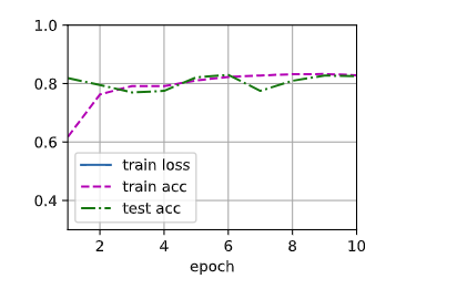
def train(num_epochs, net, train_data, test_data, loss, updater, ylim=[0.3, 1.0], need_assert=True):
"""
num_epochs: 迭代周期个数
net: 网络模型函数
train_data: 训练集
test_data: 测试集
loss: 损失函数
updater: 优化器
"""
animator = Animator(xlabel='epoch', xlim=[1, num_epochs], ylim=ylim,
legend=['train loss', 'train acc', 'test acc'])
for epoch in range(num_epochs):
train_metrics = train_epoch(train_data, net, loss, updater)
test_acc = evaluate_accuracy(net, test_data)
animator.add(epoch + 1, train_metrics + (test_acc,)) # train_metrics + (test_acc,) 是有三个元素的元组
train_loss, train_acc = train_metrics
if need_assert:
assert train_loss < 5, train_loss
assert train_acc <= 1 and train_acc > 0.5, train_acc
assert test_acc <= 1 and test_acc > 0.5, test_acc
print("train_loss:", round(train_loss, 5))
print("train_acc:", round(train_acc, 5))
print("test_acc:", round(test_acc, 5))
batch_size = 20  # 输入 X 的 X.shape[0]
num_epochs = 10  # 迭代周期数

train_dt = data_iter(train_data, batch_size)
test_dt = data_iter(test_data, batch_size)
type(train_dt), type(test_dt)
loss = cross_entropy
# updater=torch.optim.SGD([W, b], lr=0.1, momentum=0.9)
updater = sgd_updater

train(num_epochs, net, train_dt, test_dt, loss, updater)
> train_loss: 1.51878 train_acc: 0.83004 test_acc: 0.80156
12. 预测
def predict(net, test_data, n=6):
    """预测标签"""
    for X, y in test_data:
        break
    trues = y
    preds = net(X).argmax(axis=1)

    indexs = list(range(len(trues)))
    random.shuffle(indexs)
    for i in indexs[:n]:
        print("true:", y[i])
        print("pred:", preds[i])
        print("=" * 15)
predict(net, test_dt, n=5)
输出:
true: tensor(4)
pred: tensor(4)
===============
true: tensor(2)
pred: tensor(2)
===============
true: tensor(1)
pred: tensor(1)
===============
true: tensor(8)
pred: tensor(8)
===============
true: tensor(9)
pred: tensor(6)
===============
def predict_plot(net, test_data):
    """预测标签3D图"""
    for X, y in test_data:
        break
    pred_samples = collections.defaultdict(list)
    for a, b in zip(X, y):
        pred_samples[int(b)].append(a.tolist())
    sd = sorted(pred_samples.items(), key=lambda e: e[0])
    _3d_plot(collections.OrderedDict(sd))
predict_plot(net, test_dt)

13. XOR问题 (Minsky & Papert, 1969)
Q: 能不能描述一下XOR问题 (Minsky & Papert, 1969)
文心一言:在1969年,Marvin Minsky和Seymour Papert提出了一个关于单层神经网络(也称为感知机)的功能及局限性的重要观点,并以XOR问题为例进行了阐述。
XOR问题是一个简单的逻辑运算问题,其规则是:当两个输入中有一个为1且另一个为0时,输出为1;否则,输出为0。这个问题对于人类来说很简单,但对于单层神经网络来说却是一个挑战。
Minsky和Papert通过分析单层神经网络的工作原理,证明了单层神经网络无法准确解决XOR问题。单层神经网络只能产生线性分割面,而XOR问题是一个非线性问题,无法用单一的线性分割面来解决。因此,单层神经网络无法拟合XOR函数。
这个发现对神经网络的发展产生了深远的影响。它揭示了单层神经网络的局限性,并推动了多层神经网络(如深度神经网络)的研究和发展。多层神经网络通过引入隐藏层,可以产生更复杂的非线性分割面,从而解决XOR等非线性问题。
总的来说,Minsky和Papert在1969年提出的XOR问题是对单层神经网络功能及局限性的一个重要探讨,它揭示了单层神经网络的局限性,并推动了神经网络领域的发展。
我们构作一个类 XOR 样本集。生成 12 个簇,并把其中任意 4 个簇合并,使用同一种标号,此时 12 个簇一共产生 12 / 4 = 3 种标号
def gen_xor_samples(clustr_num, partition):
    samples = dict(generate_sample(clustr_num))

    indexs = [i for i in range(clustr_num)]
    random.shuffle(indexs)

    xor_samples = collections.defaultdict(list)
    for i, label in enumerate(indexs):
        xor_samples[math.floor(i / partition)] += samples[label]
    return xor_samples
clustr_num = 16
partition = 2
xor_samples = gen_xor_samples(clustr_num, partition)
# xor_samples
%matplotlib inline
_3d_plot(xor_samples)
xor_train_data, xor_test_data = load_sample(xor_samples)
# xor_train_data, xor_test_data
len(xor_train_data), len(xor_test_data)
> (8274, 2069)
nums_input = DIM  # 输入数据的维度
nums_output = math.floor(clustr_num / partition)  # CLUSTR_NUM 是标签数

W = torch.normal(0, 0.01, size=(nums_input, nums_output), requires_grad=True, dtype=torch.float64)
b = torch.zeros(nums_output, requires_grad=True, dtype=torch.float64)
batch_size = 32  # 输入 X 的 X.shape[0]
num_epochs = 10  # 迭代周期数

xor_train_dt = data_iter(xor_train_data, batch_size)
xor_test_dt = data_iter(xor_test_data, batch_size)
loss = cross_entropy
# updater=torch.optim.SGD([W, b], lr=0.1, momentum=0.9)
updater = sgd_updater
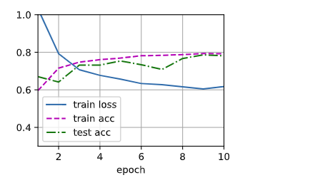
train(num_epochs, net, xor_train_dt, xor_test_dt, loss, updater, ylim=[0.0, 1.0], need_assert=False)
> train_loss: 5.7881 train_acc: 0.44816 test_acc: 0.42188
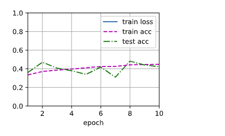
结论就是,softmax 回归拟合不了类 XOR 函数,这需要引入 多层感知机 解决。
五、softmax 回归的简洁实现
通过深度学习框架的高级API能够使实现同样的功能,并且能让我们拥有更高的编码效率。
简化了以下构建的编写:
- 网络模型(前向传播):线性方程 + softmax 算子
- 参数初始化
- loss 函数:用于计算梯度
- 优化器:用梯度更新参数
可以看到,主要构件的编写流程都被简化了
%matplotlib inline
import torch
from torch import nn
import torchvision
from torchvision import transforms
import random
import math
import numpy as np
import collections
import matplotlib.pyplot as plt
from IPython import display
1. 导入数据
def get_dataloader_workers():
    """Use 4 processes to read the data.

    Defined in :numref:`sec_utils`"""
    return 4


def load_data_fashion_mnist(batch_size, resize=None):
    """Download the Fashion-MNIST dataset and then load it into memory.

    Defined in :numref:`sec_utils`"""
    trans = [transforms.ToTensor()]
    if resize:
        trans.insert(0, transforms.Resize(resize))
    trans = transforms.Compose(trans)
    mnist_train = torchvision.datasets.FashionMNIST(
        root="../data", train=True, transform=trans, download=True)
    mnist_test = torchvision.datasets.FashionMNIST(
        root="../data", train=False, transform=trans, download=True)
    return (torch.utils.data.DataLoader(mnist_train, batch_size, shuffle=True,
                                        num_workers=get_dataloader_workers()),
            torch.utils.data.DataLoader(mnist_test, batch_size, shuffle=False,
                                        num_workers=get_dataloader_workers()))
batch_size = 256
train_iter, test_iter = load_data_fashion_mnist(batch_size)
type(train_iter), type(test_iter)
> (torch.utils.data.dataloader.DataLoader, torch.utils.data.dataloader.DataLoader)
len([e for e in train_iter])
> 235
2. 定义网络模型
# PyTorch不会隐式地调整输入的形状。因此,
# 我们在线性层前定义了展平层(flatten),来调整网络输入的形状
net = nn.Sequential(nn.Flatten(), nn.Linear(784, 10))

l = [e for e in net.parameters()]
# l
l[0].shape, l[1].shape
> (torch.Size([10, 784]), torch.Size([10]))
3. 初始化模型参数
def init_weights(m):
    if type(m) == nn.Linear:
        nn.init.normal_(m.weight, std=0.01)

net.apply(init_weights)
4. 重新审视Softmax的实现
loss = nn.CrossEntropyLoss(reduction='none')
5. 优化算法
trainer = torch.optim.SGD(net.parameters(), lr=0.1)
6. 必要构件
# 累加器
class Accumulator:
    """在n个变量上累加"""
    def __init__(self, n):
        self.data = [0.0] * n

    def add(self, *args):
        self.data = [a + float(b) for a, b in zip(self.data, args)]

    def reset(self):
        self.data = [0.0] * len(self.data)

    def __getitem__(self, idx):
        return self.data[idx]
# 训练图作图器
class Animator:
    """在动画中绘制数据"""
    def __init__(self, xlabel=None, ylabel=None, legend=None, xlim=None,
                 ylim=None, xscale='linear', yscale='linear',
                 fmts=('-', 'm--', 'g-.', 'r:'), nrows=1, ncols=1,
                 figsize=(3.5, 2.5)):
        # 增量地绘制多条线
        if legend is None:
            legend = []
        self.use_svg_display()
        self.fig, self.axes = plt.subplots(nrows, ncols, figsize=figsize)
        if nrows * ncols == 1:
            self.axes = [self.axes, ]
        # 使用lambda函数捕获参数
        self.config_axes = lambda: self.set_axes(
            self.axes[0], xlabel, ylabel, xlim, ylim, xscale, yscale, legend)
        self.X, self.Y, self.fmts = None, None, fmts

    @staticmethod
    def use_svg_display():
        """Use the svg format to display a plot in Jupyter.

        Defined in :numref:`sec_calculus`"""
        from matplotlib_inline import backend_inline
        backend_inline.set_matplotlib_formats('svg')

    @staticmethod
    def set_axes(axes, xlabel, ylabel, xlim, ylim, xscale, yscale, legend):
        """Set the axes for matplotlib.

        Defined in :numref:`sec_calculus`"""
        axes.set_xlabel(xlabel), axes.set_ylabel(ylabel)
        axes.set_xscale(xscale), axes.set_yscale(yscale)
        axes.set_xlim(xlim),     axes.set_ylim(ylim)
        if legend:
            axes.legend(legend)
        axes.grid()

    def add(self, x, y):
        # 向图表中添加多个数据点
        if not hasattr(y, "__len__"):
            y = [y]
        n = len(y)
        if not hasattr(x, "__len__"):
            x = [x] * n
        if not self.X:
            self.X = [[] for _ in range(n)]
        if not self.Y:
            self.Y = [[] for _ in range(n)]
        for i, (a, b) in enumerate(zip(x, y)):
            if a is not None and b is not None:
                self.X[i].append(a)
                self.Y[i].append(b)
        self.axes[0].cla()
        for x, y, fmt in zip(self.X, self.Y, self.fmts):
            self.axes[0].plot(x, y, fmt)
        self.config_axes()
        display.display(self.fig)
        display.clear_output(wait=True)
def accuracy(y_hat, y):
    """计算预测正确的数量"""
    if len(y_hat.shape) > 1 and y_hat.shape[1] > 1:
        y_hat = y_hat.argmax(axis=1)
    cmp = y_hat.type(y.dtype) == y
    return float(cmp.type(y.dtype).sum())
def evaluate_accuracy(net, data_iter):  #@save
    """计算在指定数据集上模型的精度"""
    if isinstance(net, torch.nn.Module):
        net.eval()  # 将模型设置为评估模式
    metric = Accumulator(2)  # 正确预测数、预测总数
    with torch.no_grad():
        for X, y in data_iter:
            metric.add(accuracy(net(X), y), y.numel())
    return metric[0] / metric[1]
7. 训练
# 单批量训练
def train_epoch(train_data, net, loss, updater):
    metric = Accumulator(4)  # 用于存储 (训练损失总和、训练准确度总和、样本数)
    for X, y in train_data:
        # print(X, y)
        # 正向传播
        y_hat = net(X)

        # 计算梯度
        l = loss(y_hat, y)

        if isinstance(updater, torch.optim.Optimizer):
            # 使用PyTorch内置的优化器和损失函数
            updater.zero_grad()
            l.mean().backward()
            updater.step()
        else:
            # 反向传播
            l.sum().backward()

            # 使用优化器,更新参数
            # print("X.grad", X.grad)
            updater(X.shape[0])  # X.shape[0] 是批量大小 (batch_size)

        # 记录当前状态
        metric.add(float(l.sum()), accuracy(y_hat, y), y.numel(), 1)

    # 返回训练损失和训练精度
    # print(metric[:], )
    return metric[0] / metric[2],  metric[1] / metric[2], metric[3]
# 多批量训练
def train(num_epochs, net, train_data, test_data, loss, updater, ylim=[0.3, 1.0], need_assert=True):
    """
    num_epochs: 迭代周期个数
    net: 网络模型函数
    train_data: 训练集
    test_data: 测试集
    loss: 损失函数
    updater: 优化器
    """
    animator = Animator(xlabel='epoch', xlim=[1, num_epochs], ylim=ylim,
                        legend=['train loss', 'train acc', 'test acc'])

    batch_num = 0
    for epoch in range(num_epochs):
        train_metrics = train_epoch(train_data, net, loss, updater)
        test_acc = evaluate_accuracy(net, test_data)
        animator.add(epoch + 1, train_metrics[:2] + (test_acc,))  # train_metrics + (test_acc,) 是有三个元素的元组
        batch_num += train_metrics[2]
    train_loss, train_acc = train_metrics[:2]
    if need_assert:
        assert train_loss < 5, train_loss
        assert train_acc <= 1 and train_acc > 0.5, train_acc
        assert test_acc <= 1 and test_acc > 0.5, test_acc
    print("train_loss:", round(train_loss, 5))
    print("train_acc:", round(train_acc, 5))
    print("test_acc:", round(test_acc, 5))
    print("batch_num:", batch_num)
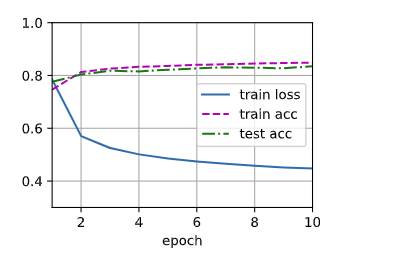
num_epochs = 10
train(num_epochs, net, train_iter, test_iter, loss, trainer)
> train_loss: 0.44763 train_acc: 0.84878 test_acc: 0.8349 batch_num: 2350.0
六、多层感知机
教程链接:mlp-scratch
%matplotlib inline
import random
import math
import numpy as np
import collections
import matplotlib.pyplot as plt
from IPython import display
import torchvision
from torchvision import transforms
import torch
from torch import nn
1. 导入 Fashion-MNIST 数据集
def get_dataloader_workers():
    """Use 4 processes to read the data.

    Defined in :numref:`sec_utils`"""
    return 4


def load_data_fashion_mnist(batch_size, resize=None):
    """Download the Fashion-MNIST dataset and then load it into memory.

    Defined in :numref:`sec_utils`"""
    trans = [transforms.ToTensor()]
    if resize:
        trans.insert(0, transforms.Resize(resize))
    trans = transforms.Compose(trans)
    mnist_train = torchvision.datasets.FashionMNIST(
        root="../data", train=True, transform=trans, download=True)
    mnist_test = torchvision.datasets.FashionMNIST(
        root="../data", train=False, transform=trans, download=True)
    return (torch.utils.data.DataLoader(mnist_train, batch_size, shuffle=True,
                                        num_workers=get_dataloader_workers()),
            torch.utils.data.DataLoader(mnist_test, batch_size, shuffle=False,
                                        num_workers=get_dataloader_workers()))
batch_size = 256
train_iter, test_iter = load_data_fashion_mnist(batch_size)
type(train_iter)
> torch.utils.data.dataloader.DataLoader
2. 初始化模型参数
num_inputs, num_outputs, num_hiddens = 784, 10, 256

W1 = nn.Parameter(torch.randn(
    num_inputs, num_hiddens, requires_grad=True) * 0.01)
b1 = nn.Parameter(torch.zeros(num_hiddens, requires_grad=True))
W2 = nn.Parameter(torch.randn(
    num_hiddens, num_outputs, requires_grad=True) * 0.01)
b2 = nn.Parameter(torch.zeros(num_outputs, requires_grad=True))

params = [W1, b1, W2, b2]
3. 激活函数
def relu(X):
    a = torch.zeros_like(X)
    return torch.max(X, a)
4. 模型
def net(X):
    X = X.reshape((-1, num_inputs))
    H = relu(X@W1 + b1)  # 这里“@”代表矩阵乘法
    return (H@W2 + b2)
5. 损失函数
loss = nn.CrossEntropyLoss(reduction='none')
6. 必要构件
# 累加器
class Accumulator:
    """在n个变量上累加"""
    def __init__(self, n):
        self.data = [0.0] * n

    def add(self, *args):
        self.data = [a + float(b) for a, b in zip(self.data, args)]

    def reset(self):
        self.data = [0.0] * len(self.data)

    def __getitem__(self, idx):
        return self.data[idx]
# 训练图作图器
class Animator:
    """在动画中绘制数据"""
    def __init__(self, xlabel=None, ylabel=None, legend=None, xlim=None,
                 ylim=None, xscale='linear', yscale='linear',
                 fmts=('-', 'm--', 'g-.', 'r:'), nrows=1, ncols=1,
                 figsize=(3.5, 2.5)):
        # 增量地绘制多条线
        if legend is None:
            legend = []
        self.use_svg_display()
        self.fig, self.axes = plt.subplots(nrows, ncols, figsize=figsize)
        if nrows * ncols == 1:
            self.axes = [self.axes, ]
        # 使用lambda函数捕获参数
        self.config_axes = lambda: self.set_axes(
            self.axes[0], xlabel, ylabel, xlim, ylim, xscale, yscale, legend)
        self.X, self.Y, self.fmts = None, None, fmts

    @staticmethod
    def use_svg_display():
        """Use the svg format to display a plot in Jupyter.

        Defined in :numref:`sec_calculus`"""
        from matplotlib_inline import backend_inline
        backend_inline.set_matplotlib_formats('svg')

    @staticmethod
    def set_axes(axes, xlabel, ylabel, xlim, ylim, xscale, yscale, legend):
        """Set the axes for matplotlib.

        Defined in :numref:`sec_calculus`"""
        axes.set_xlabel(xlabel), axes.set_ylabel(ylabel)
        axes.set_xscale(xscale), axes.set_yscale(yscale)
        axes.set_xlim(xlim),     axes.set_ylim(ylim)
        if legend:
            axes.legend(legend)
        axes.grid()

    def add(self, x, y):
        # 向图表中添加多个数据点
        if not hasattr(y, "__len__"):
            y = [y]
        n = len(y)
        if not hasattr(x, "__len__"):
            x = [x] * n
        if not self.X:
            self.X = [[] for _ in range(n)]
        if not self.Y:
            self.Y = [[] for _ in range(n)]
        for i, (a, b) in enumerate(zip(x, y)):
            if a is not None and b is not None:
                self.X[i].append(a)
                self.Y[i].append(b)
        self.axes[0].cla()
        for x, y, fmt in zip(self.X, self.Y, self.fmts):
            self.axes[0].plot(x, y, fmt)
        self.config_axes()
        display.display(self.fig)
        display.clear_output(wait=True)
def accuracy(y_hat, y):
    """计算预测正确的数量"""
    if len(y_hat.shape) > 1 and y_hat.shape[1] > 1:
        y_hat = y_hat.argmax(axis=1)
    cmp = y_hat.type(y.dtype) == y
    return float(cmp.type(y.dtype).sum())
def evaluate_accuracy(net, data_iter):  #@save
    """计算在指定数据集上模型的精度"""
    if isinstance(net, torch.nn.Module):
        net.eval()  # 将模型设置为评估模式
    metric = Accumulator(2)  # 正确预测数、预测总数
    with torch.no_grad():
        for X, y in data_iter:
            metric.add(accuracy(net(X), y), y.numel())
    return metric[0] / metric[1]
7. 训练
# 单批量训练
def train_epoch(train_data, net, loss, updater):
    metric = Accumulator(4)  # 用于存储 (训练损失总和、训练准确度总和、样本数)
    for X, y in train_data:
        # print(X, y)
        # 正向传播
        y_hat = net(X)

        # 计算梯度
        l = loss(y_hat, y)

        if isinstance(updater, torch.optim.Optimizer):
            # 使用PyTorch内置的优化器和损失函数
            updater.zero_grad()
            l.mean().backward()
            updater.step()
        else:
            # 反向传播
            l.sum().backward()

            # 使用优化器,更新参数
            # print("X.grad", X.grad)
            updater(X.shape[0])  # X.shape[0] 是批量大小 (batch_size)

        # 记录当前状态
        metric.add(float(l.sum()), accuracy(y_hat, y), y.numel(), 1)

    # 返回训练损失和训练精度
    # print(metric[:], )
    return metric[0] / metric[2],  metric[1] / metric[2], metric[3]
# 多批量训练
def train(num_epochs, net, train_data, test_data, loss, updater, ylim=[0.3, 1.0], need_assert=True):
    """
    num_epochs: 迭代周期个数
    net: 网络模型函数
    train_data: 训练集
    test_data: 测试集
    loss: 损失函数
    updater: 优化器
    """
    animator = Animator(xlabel='epoch', xlim=[1, num_epochs], ylim=ylim,
                        legend=['train loss', 'train acc', 'test acc'])

    batch_num = 0
    for epoch in range(num_epochs):
        train_metrics = train_epoch(train_data, net, loss, updater)
        test_acc = evaluate_accuracy(net, test_data)
        animator.add(epoch + 1, train_metrics[:2] + (test_acc,))  # train_metrics + (test_acc,) 是有三个元素的元组
        batch_num += train_metrics[2]
    train_loss, train_acc = train_metrics[:2]
    if need_assert:
        assert train_loss < 5, train_loss
        assert train_acc <= 1 and train_acc > 0.5, train_acc
        assert test_acc <= 1 and test_acc > 0.5, test_acc
    print("train_loss:", round(train_loss, 5))
    print("train_acc:", round(train_acc, 5))
    print("test_acc:", round(test_acc, 5))
    print("batch_num:", batch_num)
num_epochs, lr = 10, 0.1
updater = torch.optim.SGD(params, lr=lr)
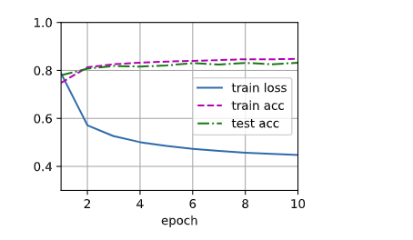
train(num_epochs, net, train_iter, test_iter, loss, updater)
> train_loss: 0.38572 train_acc: 0.86397 test_acc: 0.8497 batch_num: 2350.0
8. 预测
def predict(net, test_data, n=6):
    """预测标签"""
    for X, y in test_data:
        break
    trues = y
    preds = net(X).argmax(axis=1)

    indexs = list(range(len(trues)))
    random.shuffle(indexs)
    for i in indexs[:n]:
        print("true:", y[i])
        print("pred:", preds[i])
        print("=" * 15)
predict(net, test_iter, n=6)
输出:
true: tensor(0)
pred: tensor(0)
===============
true: tensor(1)
pred: tensor(1)
===============
true: tensor(3)
pred: tensor(3)
===============
true: tensor(3)
pred: tensor(3)
===============
true: tensor(0)
pred: tensor(0)
===============
true: tensor(1)
pred: tensor(1)
===============
⚠️ 接着我们来解决 softmax 回归一节中引入的 XOR 问题
9. 生成 样本 和 样本标号
# 画图参数
COLORS = ['b', 'g', 'r', 'c', 'm', 'y', 'k']
MARKERS = ['o', 'v', '^', 's', 'P']

# 业务参数
DIM = 3
CLUSTR_NUM = 10


def generate_sample(clustr_num, width=30, std=3, smin=600, smax=700, gen_seed=9603602):
    """生成样本
    clustr_num: 簇数
    width: 空间点位于长宽高均为 width 的正方体内
    std: 生成样本时,样本与样本中心距离的标准差
    smin: 生成样本量时,样本量的最小值
    smax: 生成样本量时,样本量的最大值
    """
    if clustr_num > len(COLORS) * len(MARKERS):
        raise Exception("Error: clustr_num <= len(COLORS) * len(MARKERS)")
    dim = DIM
    res = collections.defaultdict(list)

    random.seed(gen_seed)
    for i in range(clustr_num):
        mean = [random.random() * width for _ in range(dim)]
        sample_num = round((smax - smin) * random.random()) + smin
        for r in np.random.normal(0, std, sample_num):
            deg = [random.random() * math.pi * 2 for _ in range(2)]
            node = [mean[0] + r * math.cos(deg[0]) * math.cos(deg[1]),
                    mean[1] + r * math.cos(deg[0]) * math.sin(deg[1]),
                    mean[2] + r * math.sin(deg[0])]

            res[i].append(node)

    return res
def _3d_plot(samples):

    fig = plt.figure()
    ax = fig.add_subplot(projection='3d')

    mix = [(c, m) for c in COLORS for m in MARKERS]
    np.random.seed(19680801)
    np.random.shuffle(mix)
    for i, f in enumerate(samples.items()):
        k, v = f
        color, marker = mix[i]

        xs = [e[0] for e in v]
        ys = [e[1] for e in v]
        zs = [e[2] for e in v]
        ax.scatter(xs, ys, zs, color=color, marker=marker, label=k)

    ax.set_xlabel('X Label')
    ax.set_ylabel('Y Label')
    ax.set_zlabel('Z Label')
    ax.legend = ax.legend(bbox_to_anchor=(.5, .30, .85, .5))

    plt.show()
def gen_xor_samples(clustr_num, partition):
    samples = dict(generate_sample(clustr_num))

    indexs = [i for i in range(clustr_num)]
    random.shuffle(indexs)

    xor_samples = collections.defaultdict(list)
    for i, label in enumerate(indexs):
        xor_samples[math.floor(i / partition)] += samples[label]
    return xor_samples

clustr_num = 16
partition = 2
xor_samples = gen_xor_samples(clustr_num, partition)
# xor_samples
_3d_plot(xor_samples)
10. 分割 训练集 和 测试集
将样本字典整成元组并打乱,分成训练集和测试集
def load_sample(samples, train_rate=0.8):
    lst = []
    for y, Xlist in samples.items():
        for X in Xlist:
            lst.append((X, y))

    random.shuffle(lst)
    train_num = math.floor(len(lst) * train_rate)

    train = lst[:train_num]
    test = lst[train_num:]

    return train, test
class MyDataLoader:
    def __init__(self):
        self._lst: list
        self.i = 0

    @property
    def lst(self):
        return self._lst

    @lst.setter
    def lst(self, value):
        self._lst = value

    def __iter__(self):
        return self

    def __next__(self):
        if self.i < len(self._lst):
            i = self.i
            self.i += 1
            return self._lst[i]
        else:
            self.i = 0
            raise StopIteration


def data_iter(data, batch_size):
    """将 原始输入向量 拼接成 批量矩阵"""
    res = []
    batch_num = math.floor(len(data) / batch_size)
    for i in range(batch_num):
        start, end = batch_size * i, batch_size * (i + 1)
        # X = torch.tensor([e[0] for e in data[start:end]], requires_grad=True)
        X = torch.tensor([e[0] for e in data[start:end]])
        y = torch.tensor([e[1] for e in data[start:end]])
        res.append((X, y))

    dl = MyDataLoader()
    dl.lst = res

    return dl
xor_train_data, xor_test_data = load_sample(xor_samples)
# xor_train_data, xor_test_data
batch_size = 32
xor_train_iter = data_iter(xor_train_data, batch_size)
xor_test_iter = data_iter(xor_test_data, batch_size)
type(xor_train_iter), type(xor_test_iter)
num_inputs, num_outputs, num_hiddens = DIM, len(xor_samples.items()), 128
num_inputs, num_outputs, num_hiddens
> (3, 8, 512)
# 初始化参数
W1 = nn.Parameter(torch.randn(num_inputs, num_hiddens, requires_grad=True, dtype=torch.float64) * 0.01)
b1 = nn.Parameter(torch.zeros(num_hiddens, requires_grad=True))

W2 = nn.Parameter(torch.randn(num_hiddens, num_outputs, requires_grad=True, dtype=torch.float64) * 0.01)
b2 = nn.Parameter(torch.zeros(num_outputs, requires_grad=True))

params = [W1, b1, W2, b2]
# 激活函数
def relu(X):
    a = torch.zeros_like(X)
    return torch.max(X, a)
# 网络模型
def net(X):
    X = X.reshape((-1, num_inputs))
    H = relu(X@W1 + b1)
    return (H@W2 + b2)
# 损失函数
loss = nn.CrossEntropyLoss(reduction='none')
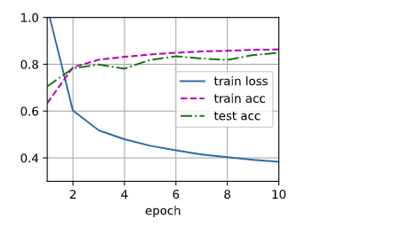
num_epochs, lr = 10, 0.1
updater = torch.optim.SGD(params, lr=lr)
train(num_epochs, net, xor_train_iter, xor_test_iter, loss, updater)
> train_loss: 0.61771 train_acc: 0.79227 test_acc: 0.78125 batch_num: 2580.0
七、多层感知机的简洁实现
%matplotlib inline
import random
import math
import numpy as np
import collections
import matplotlib.pyplot as plt
from IPython import display
import torchvision
from torchvision import transforms
import torch
from torch import nn
1. 模型
net = nn.Sequential(nn.Flatten(),
                    nn.Linear(784, 256),
                    nn.ReLU(),
                    nn.Linear(256, 10))

def init_weights(m):
    if type(m) == nn.Linear:
        nn.init.normal_(m.weight, std=0.01)

net.apply(init_weights)
def get_dataloader_workers():
    """Use 4 processes to read the data.

    Defined in :numref:`sec_utils`"""
    return 4


def load_data_fashion_mnist(batch_size, resize=None):
    """Download the Fashion-MNIST dataset and then load it into memory.

    Defined in :numref:`sec_utils`"""
    trans = [transforms.ToTensor()]
    if resize:
        trans.insert(0, transforms.Resize(resize))
    trans = transforms.Compose(trans)
    mnist_train = torchvision.datasets.FashionMNIST(
        root="../data", train=True, transform=trans, download=True)
    mnist_test = torchvision.datasets.FashionMNIST(
        root="../data", train=False, transform=trans, download=True)
    return (torch.utils.data.DataLoader(mnist_train, batch_size, shuffle=True,
                                        num_workers=get_dataloader_workers()),
            torch.utils.data.DataLoader(mnist_test, batch_size, shuffle=False,
                                        num_workers=get_dataloader_workers()))


# 累加器
class Accumulator:
    """在n个变量上累加"""
    def __init__(self, n):
        self.data = [0.0] * n

    def add(self, *args):
        self.data = [a + float(b) for a, b in zip(self.data, args)]

    def reset(self):
        self.data = [0.0] * len(self.data)

    def __getitem__(self, idx):
        return self.data[idx]


# 训练图作图器
class Animator:
    """在动画中绘制数据"""
    def __init__(self, xlabel=None, ylabel=None, legend=None, xlim=None,
                 ylim=None, xscale='linear', yscale='linear',
                 fmts=('-', 'm--', 'g-.', 'r:'), nrows=1, ncols=1,
                 figsize=(3.5, 2.5)):
        # 增量地绘制多条线
        if legend is None:
            legend = []
        self.use_svg_display()
        self.fig, self.axes = plt.subplots(nrows, ncols, figsize=figsize)
        if nrows * ncols == 1:
            self.axes = [self.axes, ]
        # 使用lambda函数捕获参数
        self.config_axes = lambda: self.set_axes(
            self.axes[0], xlabel, ylabel, xlim, ylim, xscale, yscale, legend)
        self.X, self.Y, self.fmts = None, None, fmts

    @staticmethod
    def use_svg_display():
        """Use the svg format to display a plot in Jupyter.

        Defined in :numref:`sec_calculus`"""
        from matplotlib_inline import backend_inline
        backend_inline.set_matplotlib_formats('svg')

    @staticmethod
    def set_axes(axes, xlabel, ylabel, xlim, ylim, xscale, yscale, legend):
        """Set the axes for matplotlib.

        Defined in :numref:`sec_calculus`"""
        axes.set_xlabel(xlabel), axes.set_ylabel(ylabel)
        axes.set_xscale(xscale), axes.set_yscale(yscale)
        axes.set_xlim(xlim),     axes.set_ylim(ylim)
        if legend:
            axes.legend(legend)
        axes.grid()

    def add(self, x, y):
        # 向图表中添加多个数据点
        if not hasattr(y, "__len__"):
            y = [y]
        n = len(y)
        if not hasattr(x, "__len__"):
            x = [x] * n
        if not self.X:
            self.X = [[] for _ in range(n)]
        if not self.Y:
            self.Y = [[] for _ in range(n)]
        for i, (a, b) in enumerate(zip(x, y)):
            if a is not None and b is not None:
                self.X[i].append(a)
                self.Y[i].append(b)
        self.axes[0].cla()
        for x, y, fmt in zip(self.X, self.Y, self.fmts):
            self.axes[0].plot(x, y, fmt)
        self.config_axes()
        display.display(self.fig)
        display.clear_output(wait=True)


def accuracy(y_hat, y):
    """计算预测正确的数量"""
    if len(y_hat.shape) > 1 and y_hat.shape[1] > 1:
        y_hat = y_hat.argmax(axis=1)
    cmp = y_hat.type(y.dtype) == y
    return float(cmp.type(y.dtype).sum())


def evaluate_accuracy(net, data_iter):  #@save
    """计算在指定数据集上模型的精度"""
    if isinstance(net, torch.nn.Module):
        net.eval()  # 将模型设置为评估模式
    metric = Accumulator(2)  # 正确预测数、预测总数
    with torch.no_grad():
        for X, y in data_iter:
            metric.add(accuracy(net(X), y), y.numel())
    return metric[0] / metric[1]
2. 训练
# 单批量训练
def train_epoch(train_data, net, loss, updater):
    metric = Accumulator(4)  # 用于存储 (训练损失总和、训练准确度总和、样本数)
    for X, y in train_data:
        # print(X, y)
        # 正向传播
        y_hat = net(X)

        # 计算梯度
        l = loss(y_hat, y)

        if isinstance(updater, torch.optim.Optimizer):
            # 使用PyTorch内置的优化器和损失函数
            updater.zero_grad()
            l.mean().backward()
            updater.step()
        else:
            # 反向传播
            l.sum().backward()

            # 使用优化器,更新参数
            # print("X.grad", X.grad)
            updater(X.shape[0])  # X.shape[0] 是批量大小 (batch_size)

        # 记录当前状态
        metric.add(float(l.sum()), accuracy(y_hat, y), y.numel(), 1)

    # 返回训练损失和训练精度
    # print(metric[:], )
    return metric[0] / metric[2],  metric[1] / metric[2], metric[3]


# 多批量训练
def train(num_epochs, net, train_data, test_data, loss, updater, ylim=[0.3, 1.0], need_assert=True):
    """
    num_epochs: 迭代周期个数
    net: 网络模型函数
    train_data: 训练集
    test_data: 测试集
    loss: 损失函数
    updater: 优化器
    """
    animator = Animator(xlabel='epoch', xlim=[1, num_epochs], ylim=ylim,
                        legend=['train loss', 'train acc', 'test acc'])

    batch_num = 0
    for epoch in range(num_epochs):
        train_metrics = train_epoch(train_data, net, loss, updater)
        test_acc = evaluate_accuracy(net, test_data)
        animator.add(epoch + 1, train_metrics[:2] + (test_acc,))  # train_metrics + (test_acc,) 是有三个元素的元组
        batch_num += train_metrics[2]
    train_loss, train_acc = train_metrics[:2]
    if need_assert:
        assert train_loss < 5, train_loss
        assert train_acc <= 1 and train_acc > 0.5, train_acc
        assert test_acc <= 1 and test_acc > 0.5, test_acc
    print("train_loss:", round(train_loss, 5))
    print("train_acc:", round(train_acc, 5))
    print("test_acc:", round(test_acc, 5))
    print("batch_num:", batch_num)
batch_size, lr, num_epochs = 256, 0.1, 10
loss = nn.CrossEntropyLoss(reduction='none')
trainer = torch.optim.SGD(net.parameters(), lr=lr)

train_iter, test_iter = load_data_fashion_mnist(batch_size)
train(num_epochs, net, train_iter, test_iter, loss, trainer)
> train_loss: 0.38334 train_acc: 0.86343 test_acc: 0.849 batch_num: 2350.0
八、AutoML: h2o
h2o 是一个 AutoML 框架,本节我们尝试用 h2o.automl.H2OAutoML 完成 Kaggle 竞赛 titanic.
DIRECTORY = './data'
TRAIN_FILE='titanic/train.csv'
TEST_FILE='titanic/test.csv'
MODEL_FILE='model'
PREDICT_FILE='res.csv'

LABEL_COL='Survived'
import h2o
import pandas as pd
import warnings

import util
# 隐藏 warning,请谨慎使用
warnings.filterwarnings("ignore")
1. 训练
h2o.init()
train_path = util.gen_abspath(DIRECTORY, TRAIN_FILE)
data = h2o.import_file(train_path)
data
# 处理类别变量
factor_cols = ['Name', 'Sex']
for col in factor_cols:
    data[col] = data[col].asfactor()
# 分割训练集、验证集
train, valid = data.split_frame(ratios=[0.8], seed=377)
y = LABEL_COL
x = data.columns
x.remove('PassengerId')
x.remove('Survived')
aml = h2o.automl.H2OAutoML(max_runtime_secs=1000)
aml.train(x=x, y=y, training_frame=data)
# 预测
y_pred = aml.predict(data).as_data_frame()['predict'].tolist()
y_true = data.as_data_frame()['Survived'].tolist()
y_label, threshold = util.eval_binary(y_true=y_true, y_pred=y_pred, n_trials=1000, ret=True)
输出:
threshold: 0.69676
accuracy: 1.00000
precision: 1.00000
recall: 1.00000
f1_score: 1.00000
auc: 1.00000
cross-entropy loss: 0.06207
True Positive (TP): 342
True Negative (TN): 549
False Positive (FP): 0
False Negative (FN): 0
confusion matrix:
[[549   0]
 [  0 342]]
2. 评估
# 最佳模型的表现
aml.leader.model_performance(valid)
输出:
MSE: 0.01228063484339922
RMSE: 0.11081802580536805
MAE: 0.09042077792156883
RMSLE: 0.07910391398523471
Mean Residual Deviance: 0.01228063484339922
R^2: 0.947051240897029
Null degrees of freedom: 185
Residual degrees of freedom: 183
Null deviance: 43.20171411080499
Residual deviance: 2.284198080872255
AIC: -282.5049544551409
# 最佳模型的摘要信息
aml.leader.summary()
# 特征的重要程度
aml.varimp()
# 模型排行榜
aml.leaderboard
3. 保存
# save model DIRECTORY
model_dir = util.gen_abspath(DIRECTORY, MODEL_FILE)
model_path = h2o.save_model(model=aml.leader, path=model_dir, force=True)
# load model
saved_model = h2o.load_model(model_path)
4. 预测
test_path = util.gen_abspath(DIRECTORY, TEST_FILE)
test_data = h2o.import_file(test_path)
test_data
factor_cols = ['Name', 'Sex']
for col in factor_cols:
    test_data[col] = test_data[col].asfactor()
tmp = test_data.drop(['PassengerId'], axis=1)

df_predict = aml.predict(tmp)
res = pd.DataFrame({
    'PassengerId': test_data.as_data_frame()['PassengerId'].tolist(),
    'Survived': [1 if e > threshold else 0 for e in df_predict.as_data_frame()['predict'].tolist()]
})

res
res_path = util.gen_abspath(DIRECTORY, PREDICT_FILE)
res.to_csv(res_path, index=False)
九、Hugging face
施工中…